Loans FIRE and investing Lifestyle analysis Accounting Projects Drafts About Contact

Measuring the prevalence of disease with imperfect diagnostic tests (part II)

Goals of this article

We ended part I with this statement

$$ P\left( \text{observation}|\text{hypothesis}\right) \neq P\left( \text{hypothesis}|\text{observation}\right) $$

Part I was a discussion of $P\left( \text{observation}|\text{hypothesis}\right)$. In this article we are going to explore $P\left( \text{hypothesis}|\text{observation}\right) $.

Author note

This article is heavily inspired by Keith Richards-Dinger's article. My intellectual contribution here is minimal and superficial but I think it adds some clarity. If nothing else, I improved the color choices (see bottom).

Sensitivity and specificity are the most common terms in medical diagnositic testing. They are the terms that physicians learn, the quantities the FDA wants reported, and so on. For this reason, I view using other metrics which are linear transforms of sensitivity and specificity as adding unnecessary obfuscation to any work. In reproducing Keith's results, I used sensitivity and specificity rather than false positive/negative rates. This is not an error on Keith's part. His results are still true but I feel strongly that this restatement adds clarity, particularly for physicians.

Consider the weighted coin problem backward

The probability distribution function of the true weight of a coin given $h$ heads in $n$ flips is given by a beta distribution. This is stated both by this guy and Keith. However, I do not have an authoritative source (textbook, journal article, etc) to support this claim. I think it is likely true but I am still looking for a first principles derivation to explain why it is true. That said, I will proceed assuming this is correct. I found 3blue1brown and [1] explanations of this were most useful.

Consider Bayes theorem:

$$ P(a|b) = \frac{P(b|a)P(a)}{P(b)} $$

To write a formal expression for $P\left( \text{hypothesis}|\text{observation}\right)$ we use Bayes theorem. This is called Bayesian inference and expresses the degree of certainty in the hypothesis. For $\theta$ real value, and $m$ measured value:

$$ P(\theta|m) = \frac{P(m|\theta)P(\theta)}{P(m)} $$

We already determined $P(m|\theta)$ in the previous article. The measurement $m$ here means $h$ heads in $n$ tests. Here we are using $\theta$ as the real weight of the coin

$$ P(m|\theta) = P\big( (n,h) | \theta \big) = \theta^{h} (1-\theta)^{n-h} \frac{n!}{h!\left(n-h \right)!} $$

Now we have to address $P(\theta)$. Since we know nothing about the likelyhood of the the value of $\theta$ before we do the experiment, we call this 1. This is known as a "uniform prior" in Bayesian statistics and it is somewhat contentious. That said, without this slightly handwaving-move, we don't have a way to move forward. If a sound argument can be made for a certain prior distribution, the method has more validity.

$P(m)$ is easier to handle. Since $m$ is constant no matter what hypothesis is being considered (the outcome of the experiment only happened one way), $P(m)$ is referred to as a marginal likelyhood and does not affect the "posterior probability." [1] made this point as follows:

$$ P(m) = E\big( P(m|\theta) \big) = \int P(m|\theta)P(\theta) d \theta = \text{const wrt } \theta $$

Putting it all together, we have the probability given and an experimental result.

$$ \begin{align} P(\theta|m) &= \frac{P(m|\theta)P(\theta)}{P(m)} = \\ P\big(\theta|(n,h) \big) &= \frac{P\big((n,h)|\theta\big)P(\theta)}{P\big((n,h)\big)} \\ &= \frac{ \left[ \theta^{h} (1-\theta)^{n-h} \frac{n!}{h!\left(n-h \right)!}\right] \left[1\right]}{\left[\text{const}\right]} \\ & = f(\theta) g(\text{const wrt } \theta) \end{align} $$

Everything in $g(\text{const wrt } \theta)$ is a normalization constant such that $\int_0^1P(\theta|m) d\theta = 1$. This is defined as a beta function and it is a collection of gamma functions. The gamma and beta functions here are just ways to normalize the PDF. The shape is determined by the factors from $ P(m|\theta) $ which depend on $\theta$.

$$ P\big( \theta | (n,h) \big) = \frac{\theta^h(1-\theta)^{n-h}}{B (h+1, n-h+1)} = \theta^h(1-\theta)^{n-h} \frac{ \Gamma (n+2)}{\Gamma (h+1) \Gamma (n-h+1)} $$

[Caption] Drag red dots to set the number of trials (vertical scale on the right) and the measured rate of heads (x axis). This interactive grapher implements the equation above to give the probability distribution of the true weight of a coin if $h$ heads are observed in $n$ flips.

Notice that the gamma functions are not a function of $x$. They are only there as a normalization factor for a given $n$ and $h$. Therefore we can rewrite $P(x, h, n)$ with a normalization integral instead of gamma functions.

$$ P(\theta, h, n) = \frac{ \theta^h(1-\theta)^{n-h} }{ \int_0^1 \theta^h(1-\theta)^{n-h} dx} $$

Therefore we can conclude

$$ \frac{ \Gamma (n+2)}{\Gamma (h+1) \Gamma (n-h+1)} = \int_0^1 \theta^h(1-\theta)^{n-h} dx $$

This is computationally useful because the integral expression on the right is sometimes more convenient to implement than the gamma functions on the left.

Measuring the prevalence

Let's say we did a series of three experiments to measure the disease prevalence of a population. We run the test on $x_\text{pos}$ positive patients to measure the sensitivity, $x_\text{neg}$ healthy people to measure the specificity, and $x_\text{pop}$ random members of the public to measure the prevalence. Our goal is to produce a probability distribution of the population prevalence, $P(P_\text{prev})$.

Measurement	Variable	Number of tests	Number positive
Sensitivity	$S_n$	$x_\text{pos}$	$ \lambda_\text{pos}$
Specificity	$S_p$	$x_\text{neg}$	$ \lambda_\text{neg}$
Prevalence	$P_\text{prev}$	$x_\text{pop}$	$ \lambda_\text{pop}$

Each one of these is a weighted-coin flip following the equations in the "Consider the weighted coin problem backward" section at the top. Below, we will show them without the normalizing integrals or gamma functions.

$$ \begin{align} P(S_n, x_\text{pos}, \lambda_\text{pos}) & \propto S_n^{\lambda_\text{pos}} (1-S_n)^{x_\text{pos}-\lambda_\text{pos}} \\ P(S_p, x_\text{neg}, \lambda_\text{neg}) & \propto (1-S_p)^{\lambda_\text{neg} } S_p^{x_\text{neg}-\lambda_\text{neg}} \\ P(P_\text{prev}, x_\text{pop}, \lambda_\text{pop}) & \propto \left(P_\text{prev}S_n+(1-P_\text{prev})(1-S_p)\right)^{\lambda_\text{pop}} \left(1-P_\text{prev}S_n-(1-P_\text{prev})(1-S_p) \right)^{x_\text{pop}-\lambda_\text{pop}} \end{align} $$

For any given set of experiments (ie a fixed $x_\text{pos}$, $x_\text{neg}$, $x_\text{pop}$, $ \lambda_\text{pos}$, $ \lambda_\text{neg}$, and $ \lambda_\text{pop}$) there will be a probability distribution function $P(P_\text{prev}, S_n, S_p)$ which is the product of $P(S_n) \times P(S_p) \times P(P_\text{prev})$.

$$ P(P_\text{prev}, S_n, S_p) \propto \begin{align} & \left(P_\text{prev}S_n+(1-P_\text{prev})(1-S_p)\right)^{\lambda_\text{pop}} \\ \times & \left(1-P_\text{prev}S_n-(1-P_\text{prev})(1-S_p) \right)^{x_\text{pop}-\lambda_\text{pop}} \\ \times & S_p^{\lambda_\text{neg} } (1-S_p)^{x_\text{neg}-\lambda_\text{neg}} S_n^{\lambda_\text{pos}} (1-S_n)^{x_\text{pos}-\lambda_\text{pos}} \end{align} $$

To reduce this to a function of only $P_\text{prev}$, take the double integral over $S_n$ and $S_p$ from 0 to 1. To normalize it, divide by the triple integral over $P_\text{prev}$, $S_n$ and $S_p$ from 0 to 1.

$$ P(P_\text{prev}) =\frac{\left[ \begin{align}\int_0^1 \int_0^1 &\left(P_\text{prev}S_n+(1-P_\text{prev})(1-S_p)\right)^{\lambda_\text{pop}}\\ &\left(1-P_\text{prev}S_n-(1-P_\text{prev})(1-S_p) \right)^{x_\text{pop}-\lambda_\text{pop}}\\ &(1-S_p)^{\lambda_\text{neg} } S_p^{x_\text{neg}-\lambda_\text{neg}} \\ &S_n^{\lambda_\text{pos}} (1-S_n)^{x_\text{pos}-\lambda_\text{pos}} dS_n dS_p\end{align} \right]} {\left[ \begin{align}\int_0^1 \int_0^1 \int_0^1 &\left(P_\text{prev}S_n+(1-P_\text{prev})(1-S_p)\right)^{\lambda_\text{pop}}\\ &\left(1-P_\text{prev}S_n-(1-P_\text{prev})(1-S_p) \right)^{x_\text{pop}-\lambda_\text{pop}}\\ &(1-S_p)^{\lambda_\text{neg} } S_p^{x_\text{neg}-\lambda_\text{neg}} \\ &S_n^{\lambda_\text{pos}} (1-S_n)^{x_\text{pos}-\lambda_\text{pos}} dS_n dS_p dP_\text{prev} \end{align}\right]} $$

It turns out implementing this numerically or otherwise in javascript to make a cool interactive graph is not possible. It just crashes the browser. I'm also not aware of a good way to reduce the integrals in the numerator or denominator.

Reproducing Keith's results

As stated above, this article is heavily built on Keith Richards-Dinger's work with only some slight improvements. He did the data analysis in R. I believe the Python solution is more elegant. This code reproduces the marginal 2D and 1D plots near the bottom of Keith's article under "Including uncertainties in estimates of sensitivity." He was reanalyzing statistics from [2] using the following experimental results.

Measurement	Variable	Number of tests	Number positive
Sensitivity	$S_n$	$x_\text{pos} = 122$	$ \lambda_\text{pos} = 103$
Specificity	$S_p$	$x_\text{neg} = 401$	$ \lambda_\text{neg} = 2$
Prevalence	$P_\text{prev}$	$x_\text{pop} = 3300$	$ \lambda_\text{pop}=50$

script.py

from matplotlib import cm

import numpy as np

import matplotlib.pyplot as plt

# measured results from population

xpop = 3300; lpop = 50

# measured results from known positive samples (sensitivity estimate)

xpos = 122; lpos = 103

# measured results from known negative samples (specificity estimate)

xneg = 401; lneg = 2

res = 300; #resolution of the computation (how many points?)

def joint_likely(pop, sens, spec):

p = (pop*sens + (1-pop)*(1-spec))**lpop * (1- pop*sens - (1-pop)*(1-spec))**(xpop-lpop)

pp = (1-spec)**lneg * (spec)**(xneg-lneg) * sens**lpos * (1-sens)**(xpos-lpos)

return p*pp

def confidence(x,y):

ycum = np.cumsum(y)/np.sum(y)

up = np.where(ycum > 0.9999999999)[0][0]

func = interp1d(ycum[0:up],x[0:up],'cubic');

return [func(0.025), func(0.975)]

def oneD(x,y,ax):

upper,lower = confidence(x,y)

print("95 confidence interval (%.5f,%.5f)"%(upper,lower))

ax.plot(x, y/y.sum()/(x[1]-x[0]), linewidth=2.5)

h = np.max(y/y.sum()/(x[1]-x[0]))

ax.plot([upper,lower], [h/10,h/10], linewidth=3.5, color='k')

ax.set_ylabel('Marginal PDF')

pop = np.linspace(0.00001, .04, res)

sens = np.linspace(0.601, 1, res)

spec = np.linspace(.96, 1, res)

popv, sensv, specv = np.meshgrid(pop, sens, spec)

full = joint_likely(popv, sensv, specv)

fig,axe = plt.subplots(2,3,figsize=(20,11))

ax = axe[0,0]

ax.pcolormesh(popv[1,:,:], specv[1,:,:], full.sum(axis=0), cmap=cm.viridis)

ax.set_xlabel('Prevalence'); ax.set_ylabel('Specificity')

ax = axe[0,1]

ax.pcolormesh( popv[1,:,:], sensv[:,1,:].T, full.sum(axis=2).T, cmap=cm.viridis)

ax.set_xlabel('Prevalence'); ax.set_ylabel('Sensitivity')

ax = axe[1,0]

ax.pcolormesh(specv[1,:,:],sensv[:,:,1], full.sum(axis=1), cmap=cm.viridis)

ax.set_xlabel('Specificity'); ax.set_ylabel('Sensitivity')

oneD(pop, full.sum(axis=0).sum(axis=1), axe[1,1] )

axe[1,1].set_xlabel('Prevalence')

oneD(sens, full.sum(axis=2).sum(axis=1), axe[1,2] )

axe[1,2].set_xlabel('Sensitivity')

oneD(spec, full.sum(axis=0).sum(axis=0), axe[0,2] )

axe[0,2].set_xlabel('Specificity')

plt.tight_layout()

plt.show()

>>> exec(open('keith.py').read())

95 confidence interval (0.00126,0.01903) # prevalence

95 confidence interval (0.76685,0.89622) # sensitivity

95 confidence interval (0.98572,0.99842) # specificity

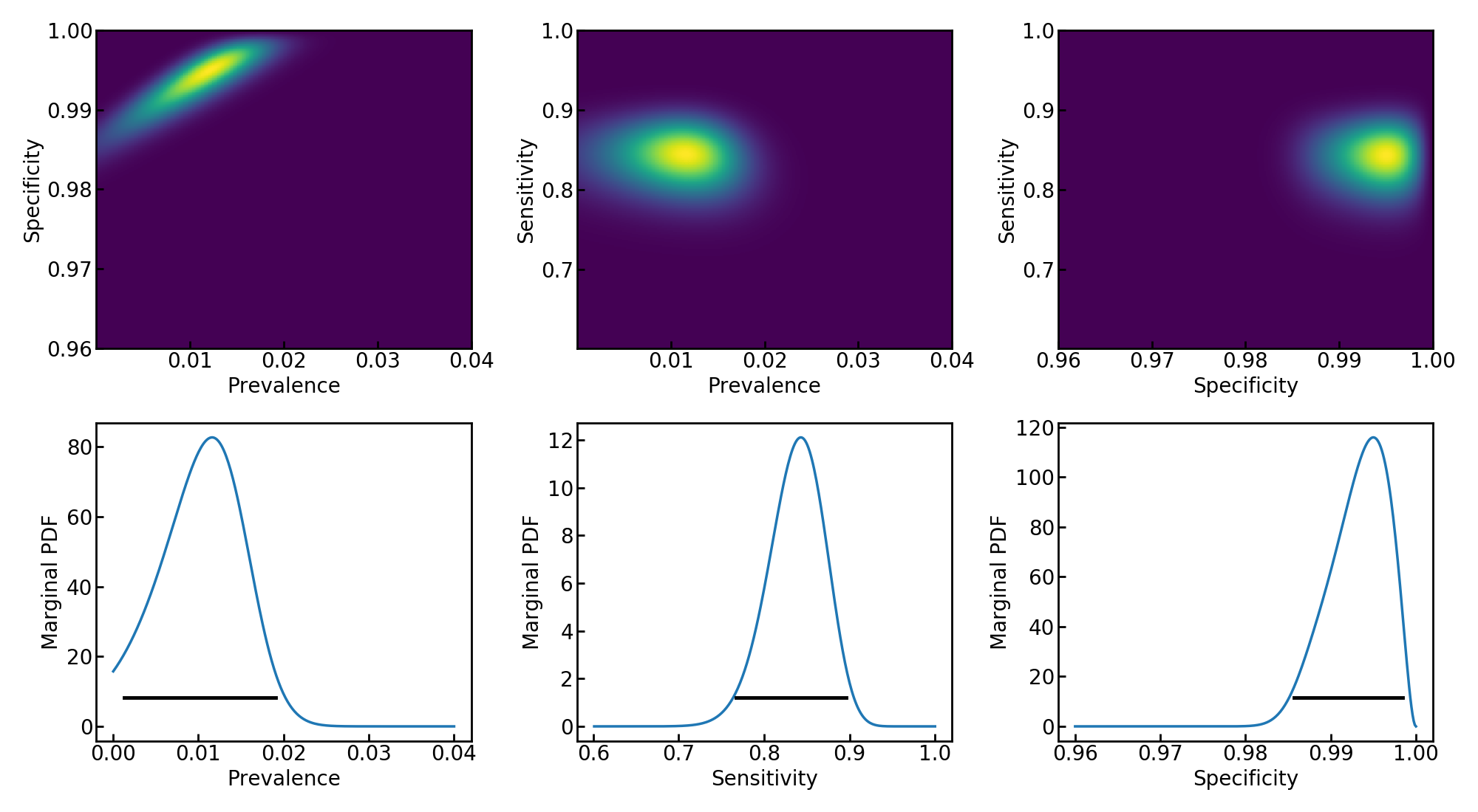
[Caption] Reproduction of Keith's 1D and 2D marginal PDF plots accounting for uncertainty in both sensitivity and specificity. These plots are mirror images of Keith's because he plotted false negative and postive rates while I plotted sensitivity and specificity.

I used the viridis color map because it is the most perceptually uniform color map I am aware of. Jet, the colormap used in Keith's images, is the default colormap in many applications but it has many shortcomings. For more information, see my brief article on colormaps.

References

[1] G. E. Box, and G. C. Tiao, "Nature of Bayesian Inference," in Bayesian Inference in Statistical Analysis, 1973.

[2] E. Bendavid, B. Mulaney, N. Sood, S. Shah, E. Ling, R. Bromley-Dulfano, C. Lai, Z. Weissberg, R. Saavedra, and J. Tedrow, "COVID-19 Antibody Seroprevalence in Santa Clara County, California," MedRxiv, 2020.

Follow @domesticengine7

Measurement	Variable	Number of tests	Number positive
Sensitivity	\(S_n\)	\(x_\text{pos}\)	\( \lambda_\text{pos}\)
Specificity	\(S_p\)	\(x_\text{neg}\)	\( \lambda_\text{neg}\)
Prevalence	\(P_\text{prev}\)	\(x_\text{pop}\)	\( \lambda_\text{pop}\)

Measurement	Variable	Number of tests	Number positive
Sensitivity	\(S_n\)	\(x_\text{pos} = 122\)	\( \lambda_\text{pos} = 103\)
Specificity	\(S_p\)	\(x_\text{neg} = 401\)	\( \lambda_\text{neg} = 2\)
Prevalence	\(P_\text{prev}\)	\(x_\text{pop} = 3300\)	\( \lambda_\text{pop}=50\)